
欢迎在文章下方评论,建议用电脑看
To the best of our knowledge, this is the first time that very deep convolutional nets have been applied to text processing.
The overall architecture of our network is shown in Figure 1. Our model begins with a look-up table that generates a 2D tensor of size (f 0 , s) that contain the embeddings of the s characters. s is fixed to 1024, and f 0 can be seen as the ”RGB” dimension of the input text.

In Figure 1, temporal convolutions with kernel size 3 and X feature maps are denoted ”3, Temp Conv, X”, fully connected layers which are linear projections (matrix of size I × O) are denoted ”fc(I, O)” and ”3-max pooling, stride 2” means temporal max pooling with kernel size 3 and stride 2.
investigated the same kind of “ResNet shortcut” connections as in (Heet al., 2016a), namely identity and 1 × 1 convolutions (see Figure 1)
Inspired by the philosophy of VGG and ResNets we apply these two design rules: (i) for the same output temporal resolution, the layers have the same number of feature maps, (ii) when the temporal resolution is halved, the number of feature maps is doubled. This helps reduce the memory footprint of the network.

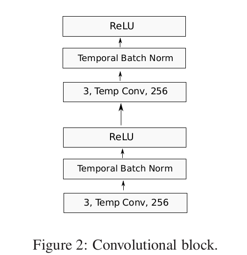
Each convolutional block (see Figure 2) is a sequence of two convolutional layers, each one followed by a temporal BatchNorm (Ioffe and Szegedy, 2015) layer and an ReLU activation.

Different depths of the overall architecture are obtained by varying the number of convolutional blocks in between the pooling layers (see table 2)
In this work, we have explored four depths for our networks: 9, 17, 29 and 49, which we define as being the number of convolutional layers. The depth of a network is obtained by summing the number of blocks with 64, 128, 256 and 512 filters, with each block containing two convolutional layers. In Figure 1, the network has 2 blocks of each type, resulting in a depth of 2 × (2 + 2 + 2 + 2) = 16. Adding the very first convolutional layer, this sums to a depth of 17 convolutional layers. The depth can thus be increased or decreased by adding or removing convolutional blocks with a certain number of filters. The best configurations we observed for depths 9, 17, 29 and 49 are described in Table 2. We also give the number of parameters of all convolutional layers.
We explore three types of down-sampling between blocks K i and K i+1 (Figure 1) :
(i) The first convolutional layer of K i+1 has stride 2 (ResNet-like).
(ii) K i is followed by a k-max pooling layer where k is such that the resolution is halved (Kalchbrenner et al., 2014).
(iii) K i is followed by max-pooling with kernel size 3 and stride 2 (VGG-like).
All these types of pooling reduce the temporal resolution by a factor 2. At the final convolutional layer, the resolution is thus s d .